Interpreting Channel Geometry Graphs
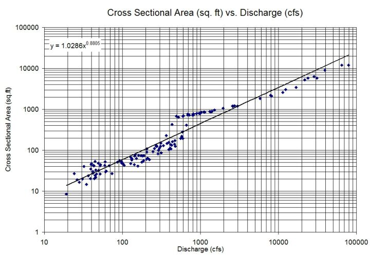
Data values included on the geometry relationships will often not have a perfect correlation. Issues to consider include when viewing these graphs are data scatter with no detectable correlation between the x and y variables, and changing data slopes between the x and y variables. Often the goal in using a geometry graphic is to read the dependent variable, or y-axis parameter, for a discharge on the x-axis. In this example, if the discharge were 1000 cfs, then the estimate of cross-sectional area could be taken as the data point or the regression line. If the data point is chosen, then read the y-intercept with that data point, and get something near 800 sq. ft. If the regression line is chosen, then enter the discharge value into the regression equation, in place of the x-variable, and compute the y-variable, which in this case is 451 sq ft. The difference between these methods is large, revealing a change in slope, rather than scatter, in this section of the graph, and the best estimate is from the data point.
| 